Analysis

Data

maindata has 60000 observations and 11 features. We are adjusting for population size by dividing val (point estimate of number of HIV/AIDS deaths) by population multiplied by 100,000 to get a mortality_per_100k variable and a log_mortality_per_100k variable.

regression = maindata %>% 
  mutate(mortality_per_100k = val / (population/100000),
         log_mortality_per_100k = log(mortality_per_100k),
         year_2004 = if_else(year <= 2004, 1, 0),
         year_2004 = as.factor(year_2004),
         country_name = as.factor(country_name)) 
regression %>% 
  summarize(col_name = colnames(regression),
            n_missing = map(regression, ~sum(is.na(.)))) %>% 
  unnest(n_missing)

## # A tibble: 14 × 2
##    col_name               n_missing
##    <chr>                      <int>
##  1 location_id                    0
##  2 country_name                   0
##  3 year                           0
##  4 gdp_per_capita              2880
##  5 population                   110
##  6 sex_id                         0
##  7 sex_name                       0
##  8 age_name                       0
##  9 val                            0
## 10 upper                          0
## 11 lower                          0
## 12 mortality_per_100k           110
## 13 log_mortality_per_100k       110
## 14 year_2004                      0

Exploratory data analysis

We will check the distribution of the following predictors: sex_name, age_name, and gdp_per_capita

Sex

sex_count = maindata %>% 
  select(country_name, population, sex_name, year) %>% 
  group_by(year, sex_name) %>% 
  distinct(population) %>% 
  mutate(count = population/100000)

In maindata, the global sex distribution across years was approximately balanced between males and females.

plot_sex = ggplot(aes(x=as.factor(year),y=count,fill=sex_name, alpha = 0.5),data=sex_count)+
  geom_bar(stat="identity") +
  ggtitle("Gender distribution across 30 years") +
  theme(axis.text.x = element_text(angle = 45, hjust = 1))+
  labs(
    x = "Year",
    y = "Count/100k population"
  )

plot_sex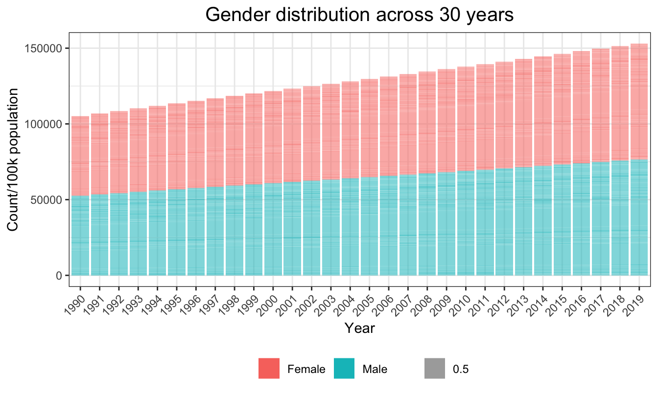

Age

age_count = maindata %>% 
  select(country_name, population, age_name, year) %>% 
  group_by(year,age_name) %>%  
  distinct(population) %>% 
  mutate(count = population/100000)

In maindata, the global age distribution across years was approximately balanced between the five age groups.

plot_age = ggplot(aes(x=as.factor(year),y=count,fill=age_name, alpha = 0.5),data=age_count)+
  geom_bar(stat="identity") +
  ggtitle("Age distribution across 30 years") +
  theme(axis.text.x = element_text(angle = 45, hjust = 1))+
  labs(
    x = "Year",
    y = "Count/100k population"
  )

plot_age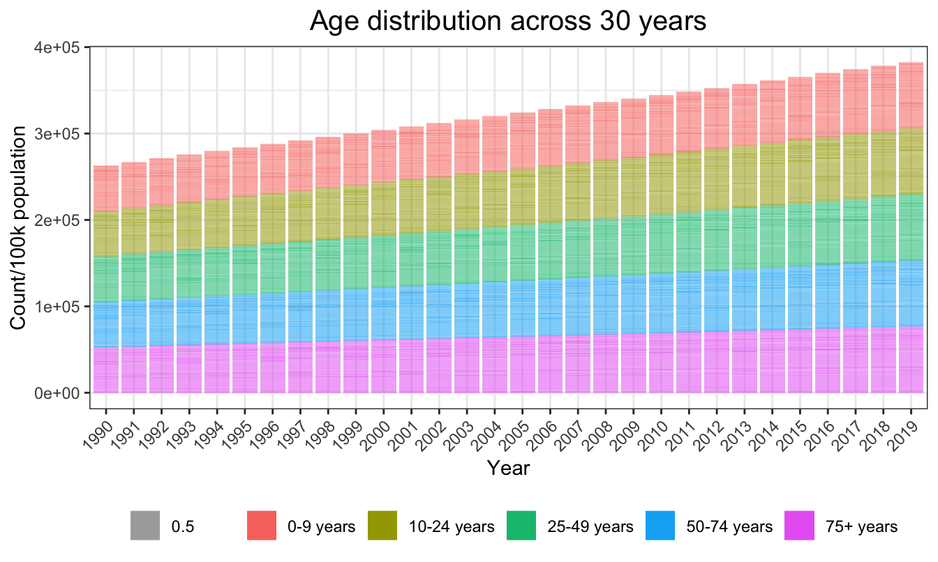

GDP per capita

gdp_count = maindata %>% 
  select(country_name, population, gdp_per_capita, year) %>% 
  group_by(year,gdp_per_capita) 

In maindata, global GDP per capita distribution was right-skewed. Most of the countries had their GDP per capita less than 10,000.

plot_gdp =  ggplot(data=maindata, aes(x=gdp_per_capita)) +
  geom_histogram(color = "darkblue", fill = "lightblue")+
  theme(axis.text.x = element_text(angle = 45, hjust = 1))+
  labs(
    title = "GDP per capita distribution in 30 years",
    x = "GDP per capita (k)",
    y = "") + 
  scale_x_continuous(
    breaks = c(0,10000,20000, 30000, 40000, 50000), 
    labels = c("0", "10k", "20k", "30k", "40k", "50k"))

plot_gdp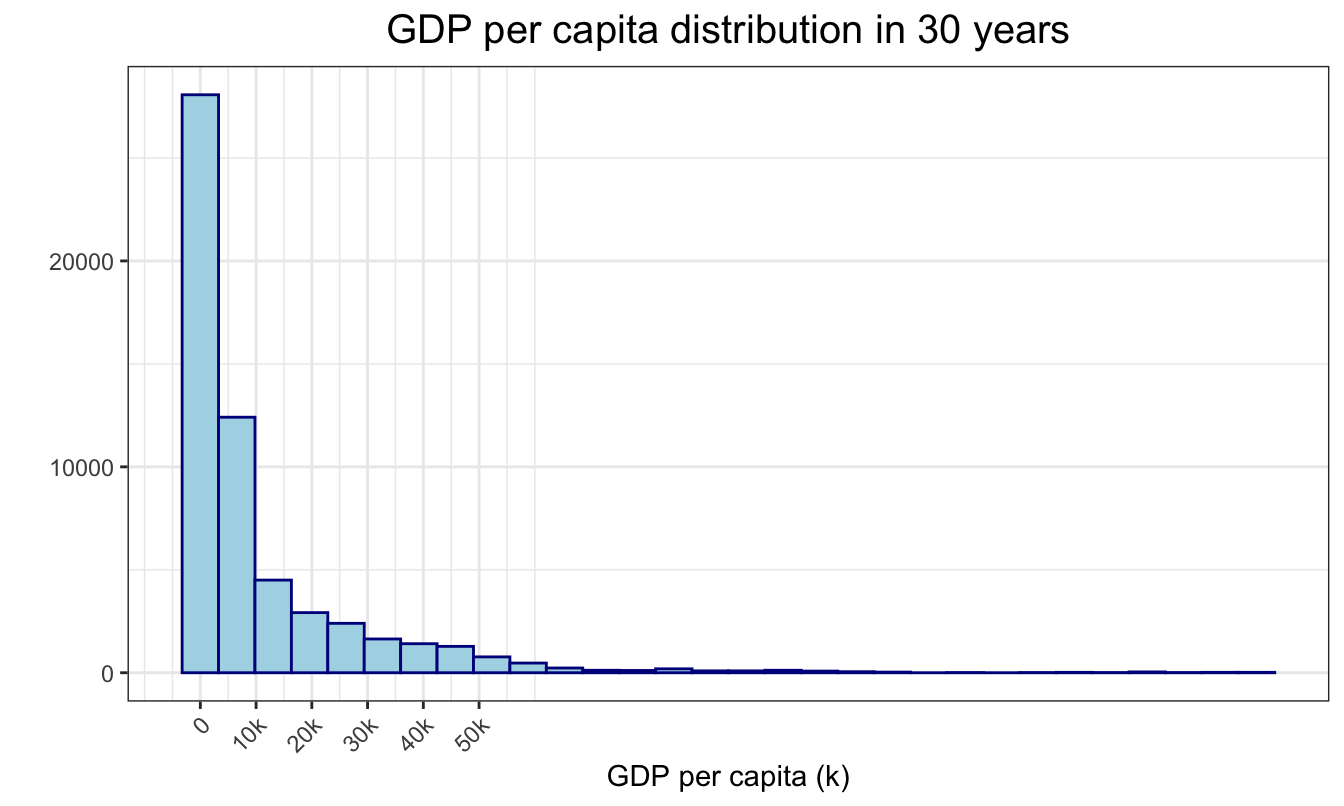

Plots of the distribution to main outcome of interest (HIV mortality per 100k population)

First, we plot the distribution of mortality_per_100k. We can see that we need to transform it to satisfy the normality assumption. So we used a log transformation to get a more normal distribution, and have a new variable mortality_per_100k.

regression %>%
 ggplot(aes(x = mortality_per_100k)) +
 geom_histogram(color = "darkblue", fill = "lightblue") +
 ggtitle("Histogram of HIV deaths per 100k") +
 geom_vline( aes(xintercept = mean(mortality_per_100k)),
            linetype = "dashed") +
 ylab("") +
 xlab("Estimated HIV deaths per 100k")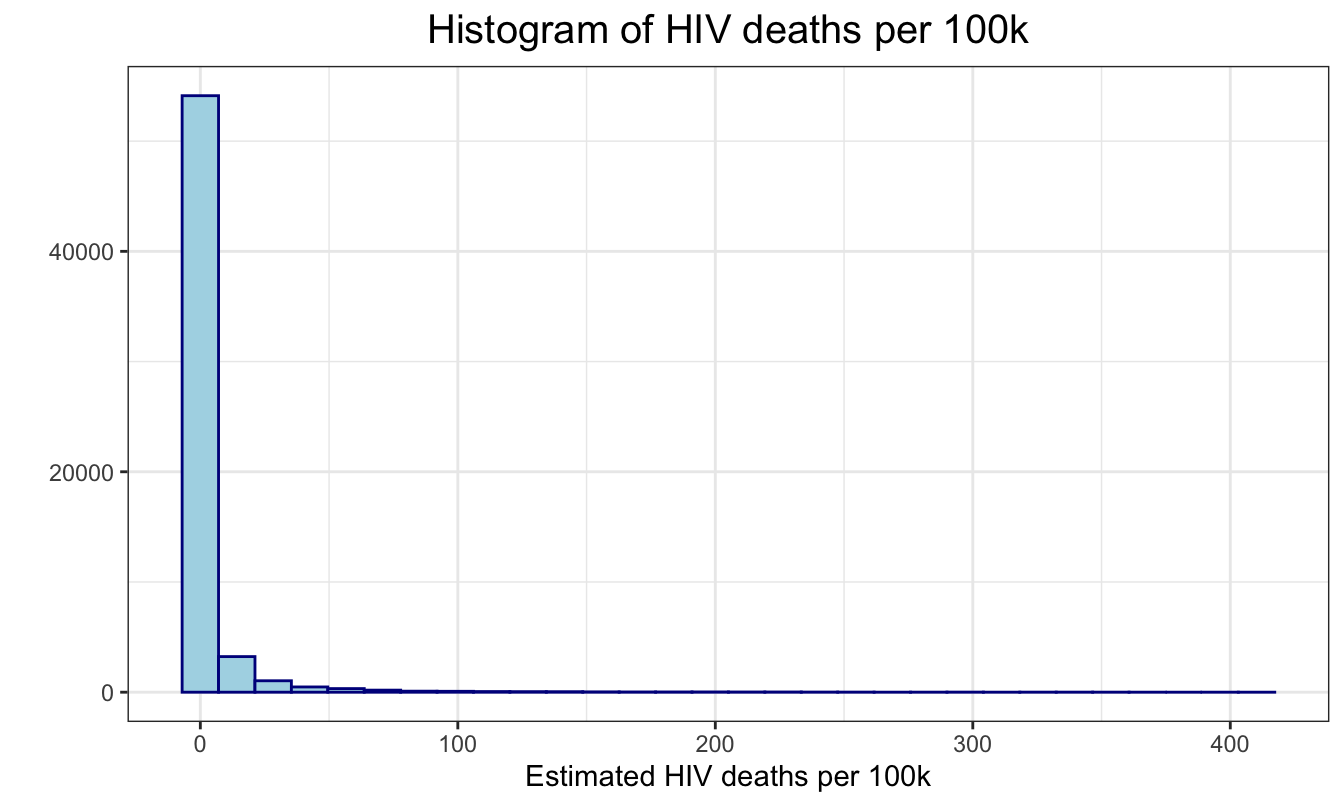

regression %>%
 ggplot(aes(x = log_mortality_per_100k)) +
 geom_histogram(color = "darkblue", fill = "lightblue") +
 ggtitle("Histogram of log(HIV deaths per 100k)") +
 geom_vline(aes(xintercept = mean(log_mortality_per_100k)),
            linetype = "dashed") +
 ylab("") +
 xlab("Estimated log(HIV deaths per 100k)")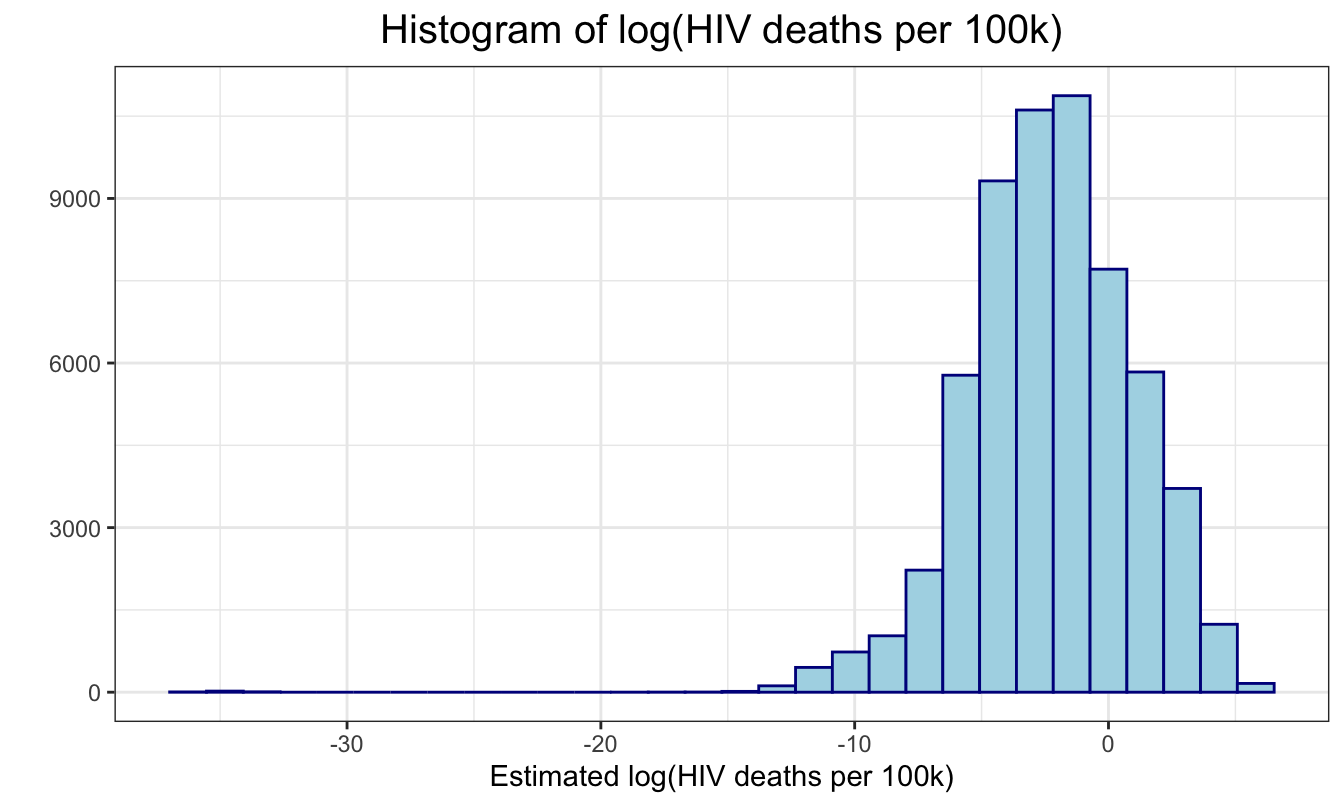

Linear regression models

Hypothesis 1

There is statistically significant relationship between the HIV deaths per 100k and age groups, sex, year, and the country’s gdp per capita respectively.

Model 1

\[ log(mortality/100000) = \beta_0 + \beta_1 age + \beta_2 sex + \beta_3 year + \beta_4 gdp \]

regression_logit = regression %>%
  mutate(log_mortality_per_100k = if_else(log_mortality_per_100k == -Inf, 0.01, log_mortality_per_100k))
  
model1_logit = lm(log_mortality_per_100k ~ age_name + sex_name + year + gdp_per_capita, data = regression_logit) %>% 
  broom::tidy() %>% 
  mutate(exp_est = exp(estimate))

model1_logit %>% 
  kable("html") %>%
  kable_styling(full_width = FALSE, position = "center") %>%
  column_spec(1:4, width = "2cm")

term	estimate	std.error	statistic	p.value	exp_est
(Intercept)	-83.4162000	2.6965462	-30.934460	0e+00	0.0000000
age_name10-24 years	-0.1839863	0.0356751	-5.157268	3e-07	0.8319472
age_name25-49 years	2.2260567	0.0356751	62.397964	0e+00	9.2632663
age_name50-74 years	0.9935827	0.0356751	27.850834	0e+00	2.7008936
age_name75+ years	-2.7893764	0.0356751	-78.188220	0e+00	0.0614595
sex_nameMale	0.4534213	0.0225629	20.095837	0e+00	1.5736870
year	0.0405708	0.0013456	30.149937	0e+00	1.0414050
gdp_per_capita	-0.0000394	0.0000006	-63.880393	0e+00	0.9999606

Interpretation: The 10-24 years old has 0.83 times the HIV mortality per 100k population compared to the 0-9 years old holding sex, year and gdp in constant. The 25-49 years old has 9.26 times the HIV mortality per 100k population compared to the 0-9 age years old holding sex, year and gdp in constant. The 50-74 years old has 2.70 times the HIV mortality per 100k population compared to the 0-9 age years old holding sex, year and gdp in constant. The 75+ years old has 0.06 times the HIV mortality per 100k population compared to the 0-9 age years old holding sex, year and gdp in constant. The HIV mortality per 100k population will increase by 4% with 1 year increase between 1990-2019 holding age, sex, and gdp in constant. The the HIV mortality per 100k population will decrease by 0.004% with 1 unit increase of gdp holding age, sex, and year in constant.

The associations between the HIV deaths per 100k and age groups, sex, year, and the country’s gdp per capita respectively are all statistically significant at the level of 5%.

Hypothesis 2

There is a significant change of the HIV deaths per 100k before and after the year 2004 controlling for age groups, sex, and gdp per capita.

Model 2

\[ log(mortality/100000) = \beta_0 + \beta_1 age + \beta_2 sex + \beta_3 year_{2004} + \beta_4gdp \]

model2_logit = lm(log_mortality_per_100k ~ age_name + sex_name + year_2004 + gdp_per_capita, data = regression_logit) %>% 
  broom::tidy() %>% 
  mutate(exp_est = exp(estimate))

model2_logit %>% 
  kable("html") %>%
  kable_styling(full_width = FALSE, position = "center") %>%
  column_spec(1:4, width = "2cm")

term	estimate	std.error	statistic	p.value	exp_est
(Intercept)	-1.8001083	0.0311420	-57.803261	0e+00	0.1652810
age_name10-24 years	-0.1839863	0.0357550	-5.145753	3e-07	0.8319472
age_name25-49 years	2.2260567	0.0357550	62.258651	0e+00	9.2632663
age_name50-74 years	0.9935827	0.0357550	27.788653	0e+00	2.7008936
age_name75+ years	-2.7893764	0.0357550	-78.013652	0e+00	0.0614595
sex_nameMale	0.4534213	0.0226134	20.050970	0e+00	1.5736870
year_20041	-0.5889625	0.0230970	-25.499530	0e+00	0.5549027
gdp_per_capita	-0.0000388	0.0000006	-62.787825	0e+00	0.9999612

Interpretation: The HIV deaths per 100k is 44.51% lower before 2004 than after 2004 after controlling for age, sex, and gdp per capita at the level of 5% significance.

Hypothesis 3

There is an interaction between age and sex.

Model 3

\[ log(mortality/100000) = \beta_0 + \beta_1 age + \beta_2 sex + \beta_3 year + \beta_4 gdp + \beta_5 age*sex \]

model1_compare = lm(log_mortality_per_100k ~ age_name + sex_name + year + gdp_per_capita, data = regression_logit)

model3_logit = lm(log_mortality_per_100k ~ age_name + sex_name + year + gdp_per_capita + age_name*sex_name, data = regression_logit) 

Anova(model1_compare, model3_logit)

## Anova Table (Type II tests)
## 
## Response: log_mortality_per_100k
##                Sum Sq    Df F value    Pr(>F)    
## age_name       157021     4 5427.12 < 2.2e-16 ***
## sex_name         2936     1  405.88 < 2.2e-16 ***
## year             6608     1  913.61 < 2.2e-16 ***
## gdp_per_capita  29666     1 4101.34 < 2.2e-16 ***
## Residuals      413073 57108                      
## ---
## Signif. codes:  0 '***' 0.001 '**' 0.01 '*' 0.05 '.' 0.1 ' ' 1

Interpretation: There is an interaction between age groups and sex at the 5% significance level, which means that gender can have different impacts on the HIV deaths per 100k regarding to different age groups.